去噪扩散概率模型 (Denoising Diffusion Probabilistic Models)

Jonathan Ho UC Berkeley jonathanho@berkeley.edu

Ajay Jain UC Berkeley ajayj@berkeley.edu

Pieter Abbeel UC Berkeley pabbeel@cs.berkeley.edu

摘要

我们展示了使用扩散概率模型（一类受非平衡热力学启发而产生的潜变量模型）进行高质量图像合成的结果。我们通过训练一个加权变分界（weighted variational bound）获得了最佳结果，该界是根据扩散概率模型与带 Langevin 动力学的去噪得分匹配（denoising score matching）之间的一种新颖联系而设计的。我们的模型自然地支持一种渐进式有损解压方案，该方案可以被解释为自回归解码的一种推广。在无条件 CIFAR10 数据集上，我们获得了 9.46 的 Inception 分数和 3.17 的业界领先 FID 分数。在 256x256 LSUN 数据集上，我们获得了与 ProgressiveGAN 相当的样本质量。我们的实现代码可在 https://github.com/hojonathanho/diffusion 获取。

1 引言

各类深度生成模型最近在多种数据模态中展现出了高质量的样本。生成对抗网络 (GANs)、自回归模型、流模型（flows）和变分自编码器 (VAEs) 已经合成了令人惊叹的图像和音频样本 [14, 27, 3, 58, 38, 25, 10, 32, 44, 57, 26, 33, 45]，并且在基于能量的建模和得分匹配方面也取得了显著进展，产生了可与 GANs 相媲美的图像 [11, 55]。

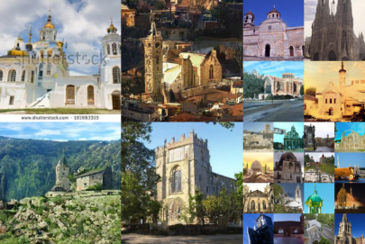
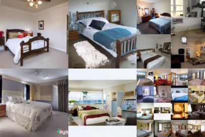
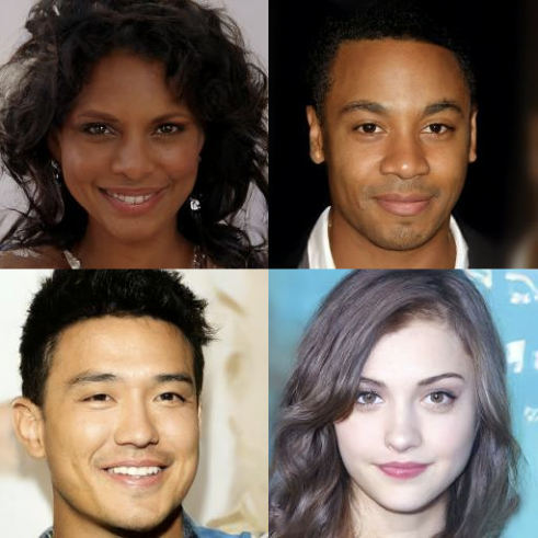图 1：CelebA-HQ 256 × 256（左）和无条件 CIFAR10（右）上的生成样本

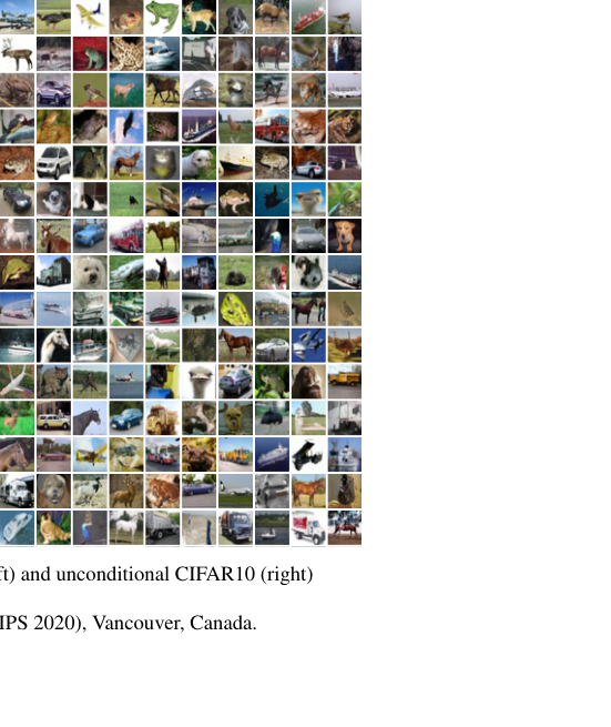图 2：本研究中考虑的定向图模型。

本文展示了扩散概率模型 [53] 的进展。扩散概率模型（为简洁起见，我们称之为“扩散模型”）是一种参数化的马尔可夫链，通过变分推理进行训练，以在有限时间后产生与数据相匹配的样本。该链的转换被学习用于反转扩散过程，扩散过程是一个马尔可夫链，它在与采样相反的方向上逐渐向数据添加噪声，直到信号被破坏。当扩散过程由少量高斯噪声组成时，将采样链的转换也设置为条件高斯分布就足够了，这允许采用一种特别简单的神经网络参数化。

扩散模型定义简单且训练高效，但据我们所知，此前尚无证据表明它们能够生成高质量样本。我们证明了扩散模型实际上能够生成高质量样本，有时甚至优于已发表的其他类型生成模型的结果（第 4 节）。此外，我们展示了扩散模型的一种特定参数化揭示了其与训练期间多噪声水平下的去噪得分匹配以及采样期间退火 Langevin 动力学之间的等价性（第 3.2 节）[55, 61]。我们使用这种参数化获得了最佳的样本质量结果（第 4.2 节），因此我们将这种等价性视为我们的主要贡献之一。

尽管样本质量很高，但与基于似然的其他模型相比，我们的模型并不具备竞争力的对数似然（不过，我们的模型对数似然优于退火重要性采样为基于能量的模型和得分匹配所报告的大估计值 [11, 55]）。我们发现，我们模型的大部分无损编码长度被用于描述难以察觉的图像细节（第 4.3 节）。我们以有损压缩的语言对这一现象进行了更深入的分析，并表明扩散模型的采样过程是一种类似于自回归解码的渐进式解码，它沿着一种位排序（bit ordering）进行，极大地推广了自回归模型通常所能实现的功能。

2 背景

扩散模型 [53] 是形式为 $p_\theta(\mathbf{x}_0) := \int p_\theta(\mathbf{x}_{0:T}) d\mathbf{x}_{1:T}$ 的潜变量模型，其中 $\mathbf{x}_1, \dots, \mathbf{x}_T$ 是与数据 $\mathbf{x}_0 \sim q(\mathbf{x}_0)$ 具有相同维度的潜变量。联合分布 $p_\theta(\mathbf{x}_{0:T})$ 被称为反向过程，它被定义为一个具有学习到的高斯转换的马尔可夫链，起始于 $p(\mathbf{x}_T) = \mathcal{N}(\mathbf{x}_T; \mathbf{0}, \mathbf{I})$ ：

$p_\theta(\mathbf{x}_{0:T}) := p(\mathbf{x}_T) \prod_{t=1}^T p_\theta(\mathbf{x}_{t-1}|\mathbf{x}_t), \quad p_\theta(\mathbf{x}_{t-1}|\mathbf{x}_t) := \mathcal{N}(\mathbf{x}_{t-1}; \boldsymbol{\mu}_\theta(\mathbf{x}_t, t), \boldsymbol{\Sigma}_\theta(\mathbf{x}_t, t)) \quad (1)$

扩散模型与其他类型潜变量模型的区别在于，近似后验 $q(\mathbf{x}_{1:T}|\mathbf{x}_0)$ （称为前向过程或扩散过程）被固定为一个马尔可夫链，根据方差调度 $\beta_1, \dots, \beta_T$ 逐渐向数据添加高斯噪声：

$q(\mathbf{x}_{1:T}|\mathbf{x}_0) := \prod_{t=1}^T q(\mathbf{x}_t|\mathbf{x}_{t-1}), \quad q(\mathbf{x}_t|\mathbf{x}_{t-1}) := \mathcal{N}(\mathbf{x}_t; \sqrt{1 - \beta_t}\mathbf{x}_{t-1}, \beta_t\mathbf{I}) \quad (2)$

训练通过优化负对数似然的常规变分界来执行：

$\mathbb{E} [-\log p_\theta(\mathbf{x}_0)] \leq \mathbb{E}_q \left[ -\log \frac{p_\theta(\mathbf{x}_{0:T})}{q(\mathbf{x}_{1:T}|\mathbf{x}_0)} \right] = \mathbb{E}_q \left[ -\log p(\mathbf{x}_T) - \sum_{t \geq 1} \log \frac{p_\theta(\mathbf{x}_{t-1}|\mathbf{x}_t)}{q(\mathbf{x}_t|\mathbf{x}_{t-1})} \right] =: L \quad (3)$

前向过程方差 $\beta_t$ 可以通过重参数化 [33] 进行学习，也可以作为超参数保持不变。反向过程的表达能力部分由 $p_\theta(\mathbf{x}_{t-1}|\mathbf{x}_t)$ 中高斯条件的选择来保证，因为当 $\beta_t$ 很小时，两个过程具有相同的函数形式 [53]。前向过程的一个显著特性是它允许以闭式形式在任意时间步 $t$ 对 $\mathbf{x}_t$ 进行采样：使用符号 $\alpha_t := 1 - \beta_t$ 和 $\bar{\alpha}_t := \prod_{s=1}^t \alpha_s$ ，我们有：

$q(\mathbf{x}_t|\mathbf{x}_0) = \mathcal{N}(\mathbf{x}_t; \sqrt{\bar{\alpha}_t}\mathbf{x}_0, (1 - \bar{\alpha}_t)\mathbf{I}) \quad (4)$

因此，通过随机梯度下降优化 $L$ 的随机项，可以实现高效训练。通过将 $L$ (3) 重写为以下形式，可以进一步通过方差缩减获得改进：

$\mathbb{E}_q [\underbrace{D_{KL}(q(\mathbf{x}_T|\mathbf{x}_0) \| p(\mathbf{x}_T))}_{L_T} + \sum_{t>1} \underbrace{D_{KL}(q(\mathbf{x}_{t-1}|\mathbf{x}_t, \mathbf{x}_0) \| p_\theta(\mathbf{x}_{t-1}|\mathbf{x}_t))}_{L_{t-1}} \underbrace{-\log p_\theta(\mathbf{x}_0|\mathbf{x}_1)}_{L_0}] \quad (5)$

（详见附录 A。各项的标签在第 3 节中使用。）公式 (5) 使用 KL 散度直接将 $p_\theta(\mathbf{x}_{t-1}|\mathbf{x}_t)$ 与前向过程后验进行比较，当以 $\mathbf{x}_0$ 为条件时，这些后验是可处理的：

$q(\mathbf{x}_{t-1}|\mathbf{x}_t, \mathbf{x}_0) = \mathcal{N}(\mathbf{x}_{t-1}; \tilde{\boldsymbol{\mu}}_t(\mathbf{x}_t, \mathbf{x}_0), \tilde{\beta}_t\mathbf{I}) \quad (6)$

其中：

$\tilde{\boldsymbol{\mu}}_t(\mathbf{x}_t, \mathbf{x}_0) := \frac{\sqrt{\bar{\alpha}_{t-1}}\beta_t}{1 - \bar{\alpha}_t}\mathbf{x}_0 + \frac{\sqrt{\alpha_t}(1 - \bar{\alpha}_{t-1})}{1 - \bar{\alpha}_t}\mathbf{x}_t \quad \text{和} \quad \tilde{\beta}_t := \frac{1 - \bar{\alpha}_{t-1}}{1 - \bar{\alpha}_t}\beta_t \quad (7)$

因此，公式 (5) 中的所有 KL 散度都是高斯分布之间的比较，因此它们可以以 Rao-Blackwellized 方式通过闭式表达式计算，而不是使用高方差的蒙特卡洛估计。

3 扩散模型与去噪自编码器

扩散模型看起来可能是一类受限的潜变量模型，但它们在实现上允许大量的自由度。人们必须选择前向过程的方差 $\beta_t$ ，以及反向过程的模型架构和高斯分布参数化。为了指导我们的选择，我们建立了扩散模型与去噪得分匹配（第 3.2 节）之间的一种新的显式联系，这导致了扩散模型的一种简化的、加权的变分界目标（第 3.4 节）。最终，我们的模型设计由简洁性和经验结果（第 4 节）证明是合理的。我们的讨论按公式 (5) 的各项进行分类。

3.1 前向过程与 $L_T$

我们忽略前向过程方差 $\beta_t$ 可通过重参数化学习的事实，而是将其固定为常数（详见第 4 节）。因此，在我们的实现中，近似后验 $q$ 没有可学习参数，因此 $L_T$ 在训练期间是一个常数，可以忽略。

3.2 反向过程与 $L_{1:T-1}$

现在我们讨论在 $1 < t \leq T$ 时 $p_\theta(\mathbf{x}_{t-1}|\mathbf{x}_t) = \mathcal{N}(\mathbf{x}_{t-1}; \boldsymbol{\mu}_\theta(\mathbf{x}_t, t), \boldsymbol{\Sigma}_\theta(\mathbf{x}_t, t))$ 的选择。首先，我们将 $\boldsymbol{\Sigma}_\theta(\mathbf{x}_t, t) = \sigma_t^2\mathbf{I}$ 设置为未经训练的时间相关常数。实验表明， $\sigma_t^2 = \beta_t$ 和 $\sigma_t^2 = \tilde{\beta}_t = \frac{1-\bar{\alpha}_{t-1}}{1-\bar{\alpha}_t}\beta_t$ 的结果相似。第一个选择对于 $\mathbf{x}_0 \sim \mathcal{N}(\mathbf{0}, \mathbf{I})$ 是最优的，第二个选择对于确定性地设置为一点的 $\mathbf{x}_0$ 是最优的。对于具有坐标单位方差的数据，这两个极端选择对应于反向过程熵的上下界 [53]。

其次，为了表示均值 $\boldsymbol{\mu}_\theta(\mathbf{x}_t, t)$ ，我们提出了一种由以下 $L_t$ 分析所激发的特定参数化。对于 $p_\theta(\mathbf{x}_{t-1}|\mathbf{x}_t) = \mathcal{N}(\mathbf{x}_{t-1}; \boldsymbol{\mu}_\theta(\mathbf{x}_t, t), \sigma_t^2\mathbf{I})$ ，我们可以写成：

$L_{t-1} = \mathbb{E}_q \left[ \frac{1}{2\sigma_t^2} \| \tilde{\boldsymbol{\mu}}_t(\mathbf{x}_t, \mathbf{x}_0) - \boldsymbol{\mu}_\theta(\mathbf{x}_t, t) \|^2 \right] + C \quad (8)$

其中 $C$ 是一个不依赖于 $\theta$ 的常数。因此，我们看到 $\boldsymbol{\mu}_\theta$ 最直接的参数化是一个预测 $\tilde{\boldsymbol{\mu}}_t$ （前向过程后验均值）的模型。然而，我们可以通过将公式 (4) 重参数化为 $\mathbf{x}_t(\mathbf{x}_0, \boldsymbol{\epsilon}) = \sqrt{\bar{\alpha}_t}\mathbf{x}_0 + \sqrt{1 - \bar{\alpha}_t}\boldsymbol{\epsilon}$ （其中 $\boldsymbol{\epsilon} \sim \mathcal{N}(\mathbf{0}, \mathbf{I})$ ）并应用前向过程后验公式 (7)，进一步展开公式 (8)：

$L_{t-1} - C = \mathbb{E}_{\mathbf{x}_0, \boldsymbol{\epsilon}} \left[ \frac{1}{2\sigma_t^2} \left\| \tilde{\boldsymbol{\mu}}_t \left( \mathbf{x}_t(\mathbf{x}_0, \boldsymbol{\epsilon}), \frac{1}{\sqrt{\bar{\alpha}_t}}(\mathbf{x}_t(\mathbf{x}_0, \boldsymbol{\epsilon}) - \sqrt{1 - \bar{\alpha}_t}\boldsymbol{\epsilon}) \right) - \boldsymbol{\mu}_\theta(\mathbf{x}_t(\mathbf{x}_0, \boldsymbol{\epsilon}), t) \right\|^2 \right] \quad (9)$ $= \mathbb{E}_{\mathbf{x}_0, \boldsymbol{\epsilon}} \left[ \frac{1}{2\sigma_t^2} \left\| \frac{1}{\sqrt{\alpha_t}} (\mathbf{x}_t(\mathbf{x}_0, \boldsymbol{\epsilon}) - \frac{\beta_t}{\sqrt{1 - \bar{\alpha}_t}}\boldsymbol{\epsilon}) - \boldsymbol{\mu}_\theta(\mathbf{x}_t(\mathbf{x}_0, \boldsymbol{\epsilon}), t) \right\|^2 \right] \quad (10)$

算法 1 训练 1: repeat 2: $\quad \mathbf{x}_0 \sim q(\mathbf{x}_0)$ 3: $\quad t \sim \text{Uniform}(\{1, \dots, T\})$ 4: $\quad \boldsymbol{\epsilon} \sim \mathcal{N}(\mathbf{0}, \mathbf{I})$ 5: $\quad$ 对 $\nabla_\theta \| \boldsymbol{\epsilon} - \boldsymbol{\epsilon}_\theta(\sqrt{\bar{\alpha}_t}\mathbf{x}_0 + \sqrt{1 - \bar{\alpha}_t}\boldsymbol{\epsilon}, t) \|^2$ 执行梯度下降步骤 6: until 收敛

算法 2 采样 1: $\mathbf{x}_T \sim \mathcal{N}(\mathbf{0}, \mathbf{I})$ 2: for $t = T, \dots, 1$ do 3: $\quad \mathbf{z} \sim \mathcal{N}(\mathbf{0}, \mathbf{I})$ 如果 $t > 1$ ，否则 $\mathbf{z} = \mathbf{0}$ 4: $\quad \mathbf{x}_{t-1} = \frac{1}{\sqrt{\alpha_t}} \left( \mathbf{x}_t - \frac{1 - \alpha_t}{\sqrt{1 - \bar{\alpha}_t}} \boldsymbol{\epsilon}_\theta(\mathbf{x}_t, t) \right) + \sigma_t \mathbf{z}$ 5: end for 6: return $\mathbf{x}_0$

公式 (10) 显示 $\boldsymbol{\mu}_\theta$ 必须在给定 $\mathbf{x}_t$ 的情况下预测 $\frac{1}{\sqrt{\alpha_t}} (\mathbf{x}_t - \frac{\beta_t}{\sqrt{1 - \bar{\alpha}_t}}\boldsymbol{\epsilon})$ 。由于 $\mathbf{x}_t$ 可作为模型的输入，我们可以选择参数化：

$\boldsymbol{\mu}_\theta(\mathbf{x}_t, t) = \tilde{\boldsymbol{\mu}}_t \left( \mathbf{x}_t, \frac{1}{\sqrt{\bar{\alpha}_t}}(\mathbf{x}_t - \sqrt{1 - \bar{\alpha}_t}\boldsymbol{\epsilon}_\theta(\mathbf{x}_t)) \right) = \frac{1}{\sqrt{\alpha_t}} \left( \mathbf{x}_t - \frac{\beta_t}{\sqrt{1 - \bar{\alpha}_t}} \boldsymbol{\epsilon}_\theta(\mathbf{x}_t, t) \right) \quad (11)$

其中 $\boldsymbol{\epsilon}_\theta$ 是一个旨在从 $\mathbf{x}_t$ 预测 $\boldsymbol{\epsilon}$ 的函数近似器。对 $\mathbf{x}_{t-1} \sim p_\theta(\mathbf{x}_{t-1}|\mathbf{x}_t)$ 进行采样，即计算 $\mathbf{x}_{t-1} = \frac{1}{\sqrt{\alpha_t}} (\mathbf{x}_t - \frac{\beta_t}{\sqrt{1 - \bar{\alpha}_t}} \boldsymbol{\epsilon}_\theta(\mathbf{x}_t, t)) + \sigma_t \mathbf{z}$ ，其中 $\mathbf{z} \sim \mathcal{N}(\mathbf{0}, \mathbf{I})$ 。完整的采样过程（算法 2）类似于 Langevin 动力学，其中 $\boldsymbol{\epsilon}_\theta$ 是学习到的数据密度梯度。此外，通过参数化 (11)，公式 (10) 简化为：

$\mathbb{E}_{\mathbf{x}_0, \boldsymbol{\epsilon}} \left[ \frac{\beta_t^2}{2\sigma_t^2 \alpha_t(1 - \bar{\alpha}_t)} \| \boldsymbol{\epsilon} - \boldsymbol{\epsilon}_\theta(\sqrt{\bar{\alpha}_t}\mathbf{x}_0 + \sqrt{1 - \bar{\alpha}_t}\boldsymbol{\epsilon}, t) \|^2 \right] \quad (12)$

这类似于在 $t$ 索引的多个噪声尺度上的去噪得分匹配 [55]。由于公式 (12) 等于（Langevin 类反向过程 (11) 的变分界的一项），我们看到优化一个类似于去噪得分匹配的目标，等同于使用变分推理来拟合类似于 Langevin 动力学的采样链的有限时间边缘分布。

总之，我们可以训练反向过程均值函数近似器 $\boldsymbol{\mu}_\theta$ 来预测 $\tilde{\boldsymbol{\mu}}_t$ ，或者通过修改其参数化，训练它来预测 $\boldsymbol{\epsilon}$ 。（也有预测 $\mathbf{x}_0$ 的可能性，但我们在实验早期发现这会导致更差的样本质量。）我们已经证明， $\boldsymbol{\epsilon}$ -预测参数化既类似于 Langevin 动力学，又简化了扩散模型的变分界，使其成为一个类似于去噪得分匹配的目标。尽管如此，它只是 $p_\theta(\mathbf{x}_{t-1}|\mathbf{x}_t)$ 的另一种参数化，因此我们在第 4 节的消融实验中验证了其有效性，我们将预测 $\boldsymbol{\epsilon}$ 与预测 $\tilde{\boldsymbol{\mu}}_t$ 进行了比较。

3.3 数据缩放、反向过程解码器与 $L_0$

我们假设图像数据由线性缩放到 $[-1, 1]$ 的 $\{0, 1, \dots, 255\}$ 中的整数组成。这确保了神经网络反向过程在从标准正态先验 $p(\mathbf{x}_T)$ 开始的一致缩放输入上运行。为了获得离散对数似然，我们将反向过程的最后一项设置为从高斯分布 $\mathcal{N}(\mathbf{x}_0; \boldsymbol{\mu}_\theta(\mathbf{x}_1, 1), \sigma_1^2\mathbf{I})$ 导出的独立离散解码器：

$p_\theta(\mathbf{x}_0|\mathbf{x}_1) = \prod_{i=1}^D \int_{\delta_-(x_0^i)}^{\delta_+(x_0^i)} \mathcal{N}(x; \mu_\theta^i(\mathbf{x}_1, 1), \sigma_1^2) dx \quad (13)$ $\delta_+(x) = \begin{cases} \infty & \text{if } x = 1 \\ x + \frac{1}{255} & \text{if } x < 1 \end{cases}, \quad \delta_-(x) = \begin{cases} -\infty & \text{if } x = -1 \\ x - \frac{1}{255} & \text{if } x > -1 \end{cases}$

其中 $D$ 是数据维度， $i$ 上标表示提取一个坐标。（直接合并更强大的解码器（如条件自回归模型）是直接的，但我们将其留给未来的工作。）类似于 VAE 解码器和自回归模型中使用的离散化连续分布 [34, 52]，我们这里的选择确保了变分界是离散数据的无损编码长度，而无需向数据添加噪声或将缩放操作的雅可比行列式纳入对数似然。在采样结束时，我们无噪声地显示 $\boldsymbol{\mu}_\theta(\mathbf{x}_1, 1)$ 。

3.4 简化训练目标

定义了上述反向过程和解码器后，由公式 (12) 和 (13) 导出的变分界显然对 $\theta$ 可微，并准备用于训练。然而，我们发现训练以下变分界的变体对样本质量有益（且更易于实现）：

$L_{\text{simple}}(\theta) := \mathbb{E}_{t, \mathbf{x}_0, \boldsymbol{\epsilon}} \left[ \| \boldsymbol{\epsilon} - \boldsymbol{\epsilon}_\theta(\sqrt{\bar{\alpha}_t}\mathbf{x}_0 + \sqrt{1 - \bar{\alpha}_t}\boldsymbol{\epsilon}, t) \|^2 \right] \quad (14)$

其中 $t$ 在 $1$ 和 $T$ 之间均匀分布。 $t=1$ 的情况对应于 $L_0$ ，其中离散解码器定义 (13) 中的积分由高斯概率密度函数乘以箱宽近似，忽略了 $\sigma_1^2$ 和边缘效应。 $t > 1$ 的情况对应于公式 (12) 的未加权版本，类似于 NCSN 去噪得分匹配模型中使用的损失加权 [55]。（ $L_T$ 不会出现，因为前向过程方差 $\beta_t$ 是固定的。）算法 1 展示了使用此简化目标的完整训练过程。

由于我们的简化目标 (14) 丢弃了公式 (12) 中的加权，它是一个加权变分界，与标准变分界相比，它强调了重构的不同方面 [18, 22]。特别是，我们在第 4 节中的扩散过程设置导致简化目标对对应于小 $t$ 的损失项进行降权。这些项训练网络去噪具有极少量噪声的数据，因此对它们进行降权是有益的，以便网络能够专注于较大 $t$ 项下更困难的去噪任务。我们将在实验中看到，这种重加权会导致更好的样本质量。

4 实验

我们将所有实验的 $T$ 设置为 1000，以便采样期间所需的神经网络评估次数与之前的工作 [53, 55] 相匹配。我们将前向过程方差设置为从 $\beta_1 = 10^{-4}$ 到 $\beta_T = 0.02$ 线性增加的常数。选择这些常数是为了相对于缩放到 $[-1, 1]$ 的数据较小，确保反向和前向过程具有大致相同的函数形式，同时保持 $\mathbf{x}_T$ 处的信噪比尽可能小（在我们的实验中， $L_T = D_{KL}(q(\mathbf{x}_T|\mathbf{x}_0) \| \mathcal{N}(\mathbf{0}, \mathbf{I})) \approx 10^{-5}$ bits/dim）。

为了表示反向过程，我们使用类似于未掩码 PixelCNN++ [52, 48] 的 U-Net 主干，并在整个过程中使用组归一化 [66]。参数在时间上共享，并通过 Transformer 正弦位置嵌入 [60] 指定给网络。我们在 $16 \times 16$ 特征图分辨率处使用自注意力 [63, 60]。详细信息见附录 B。

4.1 样本质量

表 1 显示了 CIFAR10 上的 Inception 分数、FID 分数和负对数似然（无损编码长度）。凭借 3.17 的 FID 分数，我们的无条件模型实现了比文献中大多数模型更好的样本质量，包括类条件模型。我们的 FID 分数是相对于训练集计算的，这是标准做法；当我们相对于测试集计算它时，分数为 5.24，这仍然优于文献中许多训练集 FID 分数。

6 结论

我们使用扩散模型展示了高质量的图像样本，并发现了扩散模型与用于训练马尔可夫链的变分推理、去噪得分匹配和退火 Langevin 动力学（以及扩展后的基于能量的模型）、自回归模型和渐进式有损压缩之间的联系。由于扩散模型似乎对图像数据具有极好的归纳偏置，我们期待研究它们在其他数据模态中的效用，以及作为其他类型生成模型和机器学习系统组件的潜力。

参考文献

[1] Guillaume Alain, Yoshua Bengio, Li Yao, Jason Yosinski, Eric Thibodeau-Laufer, Saizheng Zhang, and Pascal Vincent. GSNs: generative stochastic networks. Information and Inference: A Journal of the IMA, 5(2):210–249, 2016. [2] Florian Bordes, Sina Honari, and Pascal Vincent. Learning to generate samples from noise through infusion training. In International Conference on Learning Representations, 2017. [3] Andrew Brock, Jeff Donahue, and Karen Simonyan. Large scale GAN training for high fidelity natural image synthesis. In International Conference on Learning Representations, 2019. [4] Tong Che, Ruixiang Zhang, Jascha Sohl-Dickstein, Hugo Larochelle, Liam Paull, Yuan Cao, and Yoshua Bengio. Your GAN is secretly an energy-based model and you should use discriminator driven latent sampling. arXiv preprint arXiv:2003.06060, 2020. [5] Tian Qi Chen, Yulia Rubanova, Jesse Bettencourt, and David K Duvenaud. Neural ordinary differential equations. In Advances in Neural Information Processing Systems, pages 6571–6583, 2018. [6] Xi Chen, Nikhil Mishra, Mostafa Rohaninejad, and Pieter Abbeel. PixelSNAIL: An improved autoregressive generative model. In International Conference on Machine Learning, pages 863–871, 2018. [7] Rewon Child, Scott Gray, Alec Radford, and Ilya Sutskever. Generating long sequences with sparse transformers. arXiv preprint arXiv:1904.10509, 2019. [8] Yuntian Deng, Anton Bakhtin, Myle Ott, Arthur Szlam, and Marc’Aurelio Ranzato. Residual energy-based models for text generation. arXiv preprint arXiv:2004.11714, 2020. [9] Laurent Dinh, David Krueger, and Yoshua Bengio. NICE: Non-linear independent components estimation. arXiv preprint arXiv:1410.8516, 2014. [10] Laurent Dinh, Jascha Sohl-Dickstein, and Samy Bengio. Density estimation using Real NVP. arXiv preprint arXiv:1605.08803, 2016. [11] Yilun Du and Igor Mordatch. Implicit generation and modeling with energy based models. In Advances in Neural Information Processing Systems, pages 3603–3613, 2019. [12] Ruiqi Gao, Yang Lu, Junpei Zhou, Song-Chun Zhu, and Ying Nian Wu. Learning generative ConvNets via multi-grid modeling and sampling. In Proceedings of the IEEE Conference on Computer Vision and Pattern Recognition, pages 9155–9164, 2018. [13] Ruiqi Gao, Erik Nijkamp, Diederik P Kingma, Zhen Xu, Andrew M Dai, and Ying Nian Wu. Flow contrastive estimation of energy-based models. In Proceedings of the IEEE/CVF Conference on Computer Vision and Pattern Recognition, pages 7518–7528, 2020. [14] Ian Goodfellow, Jean Pouget-Abadie, Mehdi Mirza, Bing Xu, David Warde-Farley, Sherjil Ozair, Aaron Courville, and Yoshua Bengio. Generative adversarial nets. In Advances in Neural Information Processing Systems, pages 2672–2680, 2014. [15] Anirudh Goyal, Nan Rosemary Ke, Surya Ganguli, and Yoshua Bengio. Variational walkback: Learning a transition operator as a stochastic recurrent net. In Advances in Neural Information Processing Systems, pages 4392–4402, 2017. [16] Will Grathwohl, Ricky T. Q. Chen, Jesse Bettencourt, and David Duvenaud. FFJORD: Free-form continuous dynamics for scalable reversible generative models. In International Conference on Learning Representations, 2019. [17] Will Grathwohl, Kuan-Chieh Wang, Joern-Henrik Jacobsen, David Duvenaud, Mohammad Norouzi, and Kevin Swersky. Your classifier is secretly an energy based model and you should treat it like one. In International Conference on Learning Representations, 2020. [18] Karol Gregor, Frederic Besse, Danilo Jimenez Rezende, Ivo Danihelka, and Daan Wierstra. Towards conceptual compression. In Advances In Neural Information Processing Systems, pages 3549–3557, 2016. [19] Prahladh Harsha, Rahul Jain, David McAllester, and Jaikumar Radhakrishnan. The communication complexity of correlation. In Twenty-Second Annual IEEE Conference on Computational Complexity (CCC’07), pages 10–23. IEEE, 2007. [20] Marton Havasi, Robert Peharz, and José Miguel Hernández-Lobato. Minimal random code learning: Getting bits back from compressed model parameters. In International Conference on Learning Representations, 2019. [21] Martin Heusel, Hubert Ramsauer, Thomas Unterthiner, Bernhard Nessler, and Sepp Hochreiter. GANs trained by a two time-scale update rule converge to a local Nash equilibrium. In Advances in Neural Information Processing Systems, pages 6626–6637, 2017. [22] Irina Higgins, Loic Matthey, Arka Pal, Christopher Burgess, Xavier Glorot, Matthew Botvinick, Shakir Mohamed, and Alexander Lerchner. beta-VAE: Learning basic visual concepts with a constrained variational framework. In International Conference on Learning Representations, 2017. [23] Jonathan Ho, Xi Chen, Aravind Srinivas, Yan Duan, and Pieter Abbeel. Flow++: Improving flow-based generative models with variational dequantization and architecture design. In International Conference on Machine Learning, 2019. [24] Sicong Huang, Alireza Makhzani, Yanshuai Cao, and Roger Grosse. Evaluating lossy compression rates of deep generative models. In International Conference on Machine Learning, 2020. [25] Nal Kalchbrenner, Aaron van den Oord, Karen Simonyan, Ivo Danihelka, Oriol Vinyals, Alex Graves, and Koray Kavukcuoglu. Video pixel networks. In International Conference on Machine Learning, pages 1771–1779, 2017. [26] Nal Kalchbrenner, Erich Elsen, Karen Simonyan, Seb Noury, Norman Casagrande, Edward Lockhart, Florian Stimberg, Aaron van den Oord, Sander Dieleman, and Koray Kavukcuoglu. Efficient neural audio synthesis. In International Conference on Machine Learning, pages 2410–2419, 2018. [27] Tero Karras, Timo Aila, Samuli Laine, and Jaakko Lehtinen. Progressive growing of GANs for improved quality, stability, and variation. In International Conference on Learning Representations, 2018. [28] Tero Karras, Samuli Laine, and Timo Aila. A style-based generator architecture for generative adversarial networks. In Proceedings of the IEEE Conference on Computer Vision and Pattern Recognition, pages 4401–4410, 2019. [29] Tero Karras, Miika Aittala, Janne Hellsten, Samuli Laine, Jaakko Lehtinen, and Timo Aila. Training generative adversarial networks with limited data. arXiv preprint arXiv:2006.06676v1, 2020. [30] Tero Karras, Samuli Laine, Miika Aittala, Janne Hellsten, Jaakko Lehtinen, and Timo Aila. Analyzing and improving the image quality of StyleGAN. In Proceedings of the IEEE/CVF Conference on Computer Vision and Pattern Recognition, pages 8110–8119, 2020. [31] Diederik P Kingma and Jimmy Ba. Adam: A method for stochastic optimization. In International Conference on Learning Representations, 2015. [32] Diederik P Kingma and Prafulla Dhariwal. Glow: Generative flow with invertible 1x1 convolutions. In Advances in Neural Information Processing Systems, pages 10215–10224, 2018. [33] Diederik P Kingma and Max Welling. Auto-encoding variational Bayes. arXiv preprint arXiv:1312.6114, 2013. [34] Diederik P Kingma,Tim Salimans, Rafal Jozefowicz, Xi Chen, Ilya Sutskever, and Max Welling. Improved variational inference with inverse autoregressive flow. In Advances in Neural Information Processing Systems, pages 4743–4751, 2016. [35] John Lawson, George Tucker, Bo Dai, and Rajesh Ranganath. Energy-inspired models: Learning with sampler-induced distributions. In Advances in Neural Information Processing Systems, pages 8501–8513, 2019. [36] Daniel Levy, Matt D. Hoffman, and Jascha Sohl-Dickstein. Generalizing Hamiltonian Monte Carlo with neural networks. In International Conference on Learning Representations, 2018. [37] Lars Maaløe, Marco Fraccaro, Valentin Liévin, and Ole Winther. BIVA: A very deep hierarchy of latent variables for generative modeling. In Advances in Neural Information Processing Systems, pages 6548–6558, 2019. [38] Jacob Menick and Nal Kalchbrenner. Generating high fidelity images with subscale pixel networks and multidimensional upscaling. In International Conference on Learning Representations, 2019. [39] Takeru Miyato, Toshiki Kataoka, Masanori Koyama, and Yuichi Yoshida. Spectral normalization for generative adversarial networks. In International Conference on Learning Representations, 2018. [40] Alex Nichol. VQ-DRAW: A sequential discrete VAE. arXiv preprint arXiv:2003.01599, 2020. [41] Erik Nijkamp, Mitch Hill, Tian Han, Song-Chun Zhu, and Ying Nian Wu. On the anatomy of MCMC-based maximum likelihood learning of energy-based models. arXiv preprint arXiv:1903.12370, 2019. [42] Erik Nijkamp, Mitch Hill, Song-Chun Zhu, and Ying Nian Wu. Learning non-convergent non-persistent short-run MCMC toward energy-based model. In Advances in Neural Information Processing Systems, pages 5233–5243, 2019. [43] Georg Ostrovski, Will Dabney, and Remi Munos. Autoregressive quantile networks for generative modeling. In International Conference on Machine Learning, pages 3936–3945, 2018. [44] Ryan Prenger, Rafael Valle, and Bryan Catanzaro. WaveGlow: A flow-based generative network for speech synthesis. In ICASSP 2019-2019 IEEE International Conference on Acoustics, Speech and Signal Processing (ICASSP), pages 3617–3621. IEEE, 2019. [45] Ali Razavi, Aaron van den Oord, and Oriol Vinyals. Generating diverse high-fidelity images with VQ-VAE-2. In Advances in Neural Information Processing Systems, pages 14837–14847, 2019. [46] Danilo Rezende and Shakir Mohamed. Variational inference with normalizing flows. In International Conference on Machine Learning, pages 1530–1538, 2015. [47] Danilo Jimenez Rezende, Shakir Mohamed, and Daan Wierstra. Stochastic backpropagation and approximate inference in deep generative models. In International Conference on Machine Learning, pages 1278–1286, 2014. [48] Olaf Ronneberger, Philipp Fischer, and Thomas Brox. U-Net: Convolutional networks for biomedical image segmentation. In International Conference on Medical Image Computing and Computer-Assisted Intervention, pages 234–241. Springer, 2015. [49] Tim Salimans and Durk P Kingma. Weight normalization: A simple reparameterization to accelerate training of deep neural networks. In Advances in Neural Information Processing Systems, pages 901–909, 2016. [50] Tim Salimans, Diederik Kingma, and Max Welling. Markov Chain Monte Carlo and variational inference: Bridging the gap. In International Conference on Machine Learning, pages 1218–1226, 2015. [51] Tim Salimans, Ian Goodfellow, Wojciech Zaremba, Vicki Cheung, Alec Radford, and Xi Chen. Improved techniques for training gans. In Advances in Neural Information Processing Systems, pages 2234–2242, 2016. [52] Tim Salimans, Andrej Karpathy, Xi Chen, and Diederik P Kingma. PixelCNN++: Improving the PixelCNN with discretized logistic mixture likelihood and other modifications. In International Conference on Learning Representations, 2017. [53] Jascha Sohl-Dickstein, Eric Weiss, Niru Maheswaranathan, and Surya Ganguli. Deep unsupervised learning using nonequilibrium thermodynamics. In International Conference on Machine Learning, pages 2256–2265, 2015. [54] Jiaming Song, Shengjia Zhao, and Stefano Ermon. A-NICE-MC: Adversarial training for MCMC. In Advances in Neural Information Processing Systems, pages 5140–5150, 2017. [55] Yang Song and Stefano Ermon. Generative modeling by estimating gradients of the data distribution. In Advances in Neural Information Processing Systems, pages 11895–11907, 2019. [56] Yang Song and Stefano Ermon. Improved techniques for training score-based generative models. arXiv preprint arXiv:2006.09011, 2020. [57] Aaron van den Oord, Sander Dieleman, Heiga Zen, Karen Simonyan, Oriol Vinyals, Alex Graves, Nal Kalchbrenner, Andrew Senior, and Koray Kavukcuoglu. WaveNet: A generative model for raw audio. arXiv preprint arXiv:1609.03499, 2016. [58] Aaron van den Oord, Nal Kalchbrenner, and Koray Kavukcuoglu. Pixel recurrent neural networks. International Conference on Machine Learning, 2016. [59] Aaron van den Oord, Nal Kalchbrenner, Oriol Vinyals, Lasse Espeholt, Alex Graves, and Koray Kavukcuoglu. Conditional image generation with PixelCNN decoders. In Advances in Neural Information Processing Systems, pages 4790–4798, 2016. [60] Ashish Vaswani, Noam Shazeer, Niki Parmar, Jakob Uszkoreit, Llion Jones, Aidan N Gomez, Łukasz Kaiser, and Illia Polosukhin. Attention is all you need. In Advances in Neural Information Processing Systems, pages 5998–6008, 2017. [61] Pascal Vincent. A connection between score matching and denoising autoencoders. Neural Computation, 23(7):1661–1674, 2011. [62] Sheng-Yu Wang, Oliver Wang, Richard Zhang, Andrew Owens, and Alexei A Efros. Cnn-generated images are surprisingly easy to spot...for now. In Proceedings of the IEEE Conference on Computer Vision and Pattern Recognition, 2020. [63] Xiaolong Wang, Ross Girshick, Abhinav Gupta, and Kaiming He. Non-local neural networks. In Proceedings of the IEEE Conference on Computer Vision and Pattern Recognition, pages 7794–7803, 2018. [64] Auke J Wiggers and Emiel Hoogeboom. Predictive sampling with forecasting autoregressive models. arXiv preprint arXiv:2002.09928, 2020. [65] Hao Wu, Jonas Köhler, and Frank Noé. Stochastic normalizing flows. arXiv preprint arXiv:2002.06707, 2020. [66] Yuxin Wu and Kaiming He. Group normalization. In Proceedings of the European Conference on Computer Vision (ECCV), pages 3–19, 2018. [67] Jianwen Xie, Yang Lu, Song-Chun Zhu, and Yingnian Wu. A theory of generative convnet. In International Conference on Machine Learning, pages 2635–2644, 2016. [68] Jianwen Xie, Song-Chun Zhu, and Ying Nian Wu. Synthesizing dynamic patterns by spatial-temporal generative convnet. In Proceedings of the IEEE Conference on Computer Vision and Pattern Recognition, pages 7093–7101, 2017. [69] Jianwen Xie, Zilong Zheng, Ruiqi Gao, Wenguan Wang, Song-Chun Zhu, and Ying Nian Wu. Learning descriptor networks for 3d shape synthesis and analysis. In Proceedings of the IEEE Conference on Computer Vision and Pattern Recognition, pages 8629–8638, 2018. [70] Jianwen Xie, Song-Chun Zhu, and Ying Nian Wu. Learning energy-based spatial-temporal generative convnets for dynamic patterns. IEEE Transactions on Pattern Analysis and Machine Intelligence, 2019. [71] Fisher Yu, Yinda Zhang, Shuran Song, Ari Seff, and Jianxiong Xiao. LSUN: Construction of a large-scale image dataset using deep learning with humans in the loop. arXiv preprint arXiv:1506.03365, 2015. [72] Sergey Zagoruyko and Nikos Komodakis. Wide residual networks. arXiv preprint arXiv:1605.07146, 2016.

附录

额外信息

LSUN 数据集的 FID 分数包含在表 3 中。标有 * 的分数由 StyleGAN2 作为基线报告，其他分数由其各自作者报告。

模型	LSUN Bedroom	LSUN Church	LSUN Cat
ProgressiveGAN [27]	8.34	6.42	37.52
StyleGAN [28]	2.65	4.21*	8.53*
StyleGAN2 [30]	-	3.86	6.93
Ours ( $L_{\text{simple}}$ )	6.36	7.89	19.75
Ours ( $L_{\text{simple}}$ , large)	4.90	-	-

渐进式压缩 我们在第 4.3 节中的有损压缩论证仅是一个概念验证，因为算法 3 和 4 依赖于诸如最小随机编码 [20] 之类的过程，这对于高维数据是不可处理的。这些算法仅作为 Sohl-Dickstein 等人 [53] 变分界 (5) 的一种压缩解释，尚非实用的压缩系统。

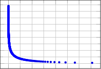
反向过程时间 ( $T - t + 1$ )	速率 (bits/dim)	失真 (RMSE [0, 255])
1000	1.77581	0.95136
900	0.11994	12.02277
800	0.05415	18.47482
700	0.02866	24.43656
600	0.01507	30.80948
500	0.00716	38.03236
400	0.00282	46.12765
300	0.00081	54.18826
200	0.00013	60.97170
100	0.00000	67.60125

A 扩展推导

以下是公式 (5) 的推导，即扩散模型的降方差变分界。该材料来自 Sohl-Dickstein 等人 [53]；我们在此仅为完整性起见将其包含在内。

$L = \mathbb{E}_q \left[ -\log \frac{p_\theta(\mathbf{x}_{0:T})}{q(\mathbf{x}_{1:T}|\mathbf{x}_0)} \right] \quad (17)$ $= \mathbb{E}_q \left[ -\log p(\mathbf{x}_T) - \sum_{t \geq 1} \log \frac{p_\theta(\mathbf{x}_{t-1}|\mathbf{x}_t)}{q(\mathbf{x}_t|\mathbf{x}_{t-1})} \right] \quad (18)$ $= \mathbb{E}_q \left[ -\log p(\mathbf{x}_T) - \sum_{t > 1} \log \frac{p_\theta(\mathbf{x}_{t-1}|\mathbf{x}_t)}{q(\mathbf{x}_t|\mathbf{x}_{t-1})} - \log \frac{p_\theta(\mathbf{x}_0|\mathbf{x}_1)}{q(\mathbf{x}_1|\mathbf{x}_0)} \right] \quad (19)$ $= \mathbb{E}_q \left[ -\log p(\mathbf{x}_T) - \sum_{t > 1} \log \frac{p_\theta(\mathbf{x}_{t-1}|\mathbf{x}_t)}{q(\mathbf{x}_{t-1}|\mathbf{x}_t, \mathbf{x}_0)} \cdot \frac{q(\mathbf{x}_{t-1}|\mathbf{x}_0)}{q(\mathbf{x}_t|\mathbf{x}_0)} - \log \frac{p_\theta(\mathbf{x}_0|\mathbf{x}_1)}{q(\mathbf{x}_1|\mathbf{x}_0)} \right] \quad (20)$ $= \mathbb{E}_q \left[ -\log \frac{p(\mathbf{x}_T)}{q(\mathbf{x}_T|\mathbf{x}_0)} - \sum_{t > 1} \log \frac{p_\theta(\mathbf{x}_{t-1}|\mathbf{x}_t)}{q(\mathbf{x}_{t-1}|\mathbf{x}_t, \mathbf{x}_0)} - \log p_\theta(\mathbf{x}_0|\mathbf{x}_1) \right] \quad (21)$ $= \mathbb{E}_q \left[ D_{KL}(q(\mathbf{x}_T|\mathbf{x}_0) \| p(\mathbf{x}_T)) + \sum_{t > 1} D_{KL}(q(\mathbf{x}_{t-1}|\mathbf{x}_t, \mathbf{x}_0) \| p_\theta(\mathbf{x}_{t-1}|\mathbf{x}_t)) - \log p_\theta(\mathbf{x}_0|\mathbf{x}_1) \right] \quad (22)$

以下是 $L$ 的另一个版本。它不可处理以进行估计，但对我们在第 4.3 节中的讨论很有用。

$L = \mathbb{E}_q \left[ -\log p(\mathbf{x}_T) - \sum_{t \geq 1} \log \frac{p_\theta(\mathbf{x}_{t-1}|\mathbf{x}_t)}{q(\mathbf{x}_t|\mathbf{x}_{t-1})} \right] \quad (23)$ $= \mathbb{E}_q \left[ -\log p(\mathbf{x}_T) - \sum_{t \geq 1} \log \frac{p_\theta(\mathbf{x}_{t-1}|\mathbf{x}_t)}{q(\mathbf{x}_{t-1}|\mathbf{x}_t)} \cdot \frac{q(\mathbf{x}_{t-1})}{q(\mathbf{x}_t)} \right] \quad (24)$ $= \mathbb{E}_q \left[ -\log \frac{p(\mathbf{x}_T)}{q(\mathbf{x}_T)} - \sum_{t \geq 1} \log \frac{p_\theta(\mathbf{x}_{t-1}|\mathbf{x}_t)}{q(\mathbf{x}_{t-1}|\mathbf{x}_t)} - \log q(\mathbf{x}_0) \right] \quad (25)$ $= D_{KL}(q(\mathbf{x}_T) \| p(\mathbf{x}_T)) + \mathbb{E}_q \left[ \sum_{t \geq 1} D_{KL}(q(\mathbf{x}_{t-1}|\mathbf{x}_t) \| p_\theta(\mathbf{x}_{t-1}|\mathbf{x}_t)) \right] + H(\mathbf{x}_0) \quad (26)$

B 实验细节

我们的神经网络架构遵循 PixelCNN++ [52] 的主干，这是一个基于 Wide ResNet [72] 的 U-Net [48]。我们用组归一化 [66] 替换了权重归一化 [49]，以使实现更简单。我们的 $32 \times 32$ 模型使用四种特征图分辨率（ $32 \times 32$ 到 $4 \times 4$ ），我们的 $256 \times 256$ 模型使用六种。所有模型在每个分辨率级别都有两个卷积残差块，并在卷积块之间在 $16 \times 16$ 分辨率处有自注意力块 [6]。扩散时间 $t$ 通过将 Transformer 正弦位置嵌入 [60] 添加到每个残差块中来指定。我们的 CIFAR10 模型有 3570 万个参数，我们的 LSUN 和 CelebA-HQ 模型有 1.14 亿个参数。我们还通过增加滤波器数量训练了一个更大的 LSUN Bedroom 模型变体，参数约为 2.56 亿。

我们对所有实验使用了 TPU v3-8（类似于 8 个 V100 GPU）。我们的 CIFAR 模型以每秒 21 步的速度训练，批大小为 128（在 800k 步完成训练需要 10.6 小时），采样 256 张图像的批次需要 17 秒。我们的 CelebA-HQ/LSUN ( $256^2$ ) 模型以每秒 2.2 步的速度训练，批大小为 64，采样 128 张图像的批次需要 300 秒。我们在 CelebA-HQ 上训练了 0.5M 步，LSUN Bedroom 2.4M 步，LSUN Cat 1.8M 步，LSUN Church 1.2M 步。更大的 LSUN Bedroom 模型训练了 1.15M 步。

除了早期为了使网络大小符合内存限制而进行的初步超参数选择外，我们进行了大部分超参数搜索以优化 CIFAR10 的样本质量，然后将所得设置转移到其他数据集：

我们从一组常数、线性和二次调度中选择了 $\beta_t$ 调度，所有调度都受到 $L_T \approx 0$ 的约束。我们设置 $T = 1000$ 而没有进行扫描，并选择了从 $\beta_1 = 10^{-4}$ 到 $\beta_T = 0.02$ 的线性调度。
我们通过在 $\{0.1, 0.2, 0.3, 0.4\}$ 的值上进行扫描，将 CIFAR10 上的 dropout 率设置为 0.1。在 CIFAR10 上没有 dropout 时，我们得到了较差的样本，让人想起未正则化的 PixelCNN++ [52] 中的过拟合伪影。我们将其他数据集上的 dropout 率设置为零，没有进行扫描。
我们在 CIFAR10 的训练期间使用了随机水平翻转；我们尝试了有翻转和无翻转的训练，发现翻转稍微提高了样本质量。除了 LSUN Bedroom 外，我们还对所有其他数据集使用了随机水平翻转。
我们在实验过程早期尝试了 Adam [31] 和 RMSProp，并选择了前者。我们将超参数保留为其标准值。我们将学习率设置为 $2 \times 10^{-4}$ 而没有进行任何扫描，并将其降低到 $2 \times 10^{-5}$ 用于 $256 \times 256$ 图像，这在较大的学习率下训练似乎不稳定。
我们将 CIFAR10 的批大小设置为 128，较大图像设置为 64。我们没有对这些值进行扫描。
我们在模型参数上使用了 EMA，衰减因子为 0.9999。我们没有对该值进行扫描。

最终实验训练了一次，并在整个训练过程中评估了样本质量。样本质量分数和对数似然报告为训练过程中的最小 FID 值。在 CIFAR10 上，我们分别使用来自 OpenAI [51] 和 TTUR [21] 存储库的原始代码计算了 50000 个样本的 Inception 和 FID 分数。在 LSUN 上，我们使用来自 StyleGAN2 [30] 存储库的代码计算了 50000 个样本的 FID 分数。CIFAR10 和 CelebA-HQ 是按照 TensorFlow Datasets (https://www.tensorflow.org/datasets) 提供的方式加载的，LSUN 是使用 StyleGAN 的代码准备的。数据集拆分（或缺乏拆分）是引入其在生成建模上下文中使用的论文的标准。所有详细信息都可以在源代码发布中找到。

C 关于相关工作的讨论

我们的模型架构、前向过程定义和先验在微妙但重要的方式上与 NCSN [55, 56] 不同，这些方式提高了样本质量，值得注意的是，我们直接将我们的采样器训练为潜变量模型，而不是在训练后事后添加它。更详细地说：

我们使用带有自注意力的 U-Net；NCSN 使用带有扩张卷积的 RefineNet。我们通过添加 Transformer 正弦位置嵌入来对所有层进行 $t$ 条件化，而不是仅在归一化层 (NCSNv1) 或仅在输出 (v2) 中。
扩散模型在每个前向过程步骤中缩小数据（通过 $\sqrt{1 - \beta_t}$ 因子），因此在添加噪声时方差不会增加，从而为神经网络反向过程提供了一致缩放的输入。NCSN 省略了此缩放因子。
与 NCSN 不同，我们的前向过程会破坏信号 ( $D_{KL}(q(\mathbf{x}_T|\mathbf{x}_0) \| \mathcal{N}(\mathbf{0}, \mathbf{I})) \approx 0$ )，确保先验与 $\mathbf{x}_T$ 的聚合后验紧密匹配。也与 NCSN 不同，我们的 $\beta_t$ 非常小，这确保了前向过程可以通过具有条件高斯分布的马尔可夫链进行反转。这两个因素都防止了采样时的分布偏移。
我们的 Langevin 类采样器具有从前向过程中的 $\beta_t$ 严格导出的系数（学习率、噪声尺度等）。因此，我们的训练过程直接训练我们的采样器以在 $T$ 步后匹配数据分布：它使用变分推理将采样器训练为潜变量模型。相比之下，NCSN 的采样器系数是事后手动设置的，并且不能保证其训练过程直接优化其采样器的质量指标。

D 样本

附加样本 图 11、13、16、17、18 和 19 显示了在 CelebA-HQ、CIFAR10 和 LSUN 数据集上训练的扩散模型的未整理样本。

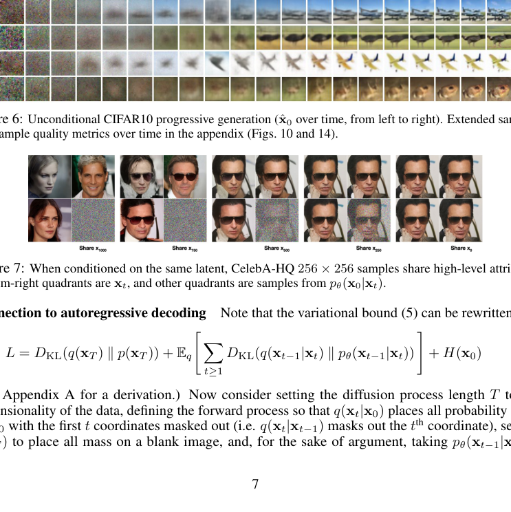
潜结构和反向过程随机性 在采样期间，先验 $\mathbf{x}_T \sim \mathcal{N}(\mathbf{0}, \mathbf{I})$ 和 Langevin 动力学都是随机的。为了理解第二个噪声源的重要性，我们为 CelebA $256 \times 256$ 数据集对以相同中间潜变量为条件的多个图像进行了采样。图 7 显示了来自反向过程 $\mathbf{x}_0 \sim p_\theta(\mathbf{x}_0|\mathbf{x}_t)$ 的多个抽取，它们共享 $t \in \{1000, 750, 500, 250\}$ 的潜变量 $\mathbf{x}_t$ 。为了实现这一点，我们从先验的初始抽取开始运行单个反向链。在中间时间步，链被拆分以采样多个图像。当链在 $\mathbf{x}_T=1000$ 的先验抽取后被拆分时，样本差异很大。然而，当链在更多步骤后被拆分时，样本共享诸如性别、头发颜色、眼镜、饱和度、姿势和面部表情等高级属性。这表明像 $\mathbf{x}_{750}$ 这样的中间潜变量尽管难以察觉，但编码了这些属性。

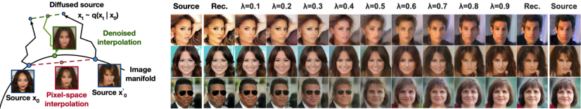
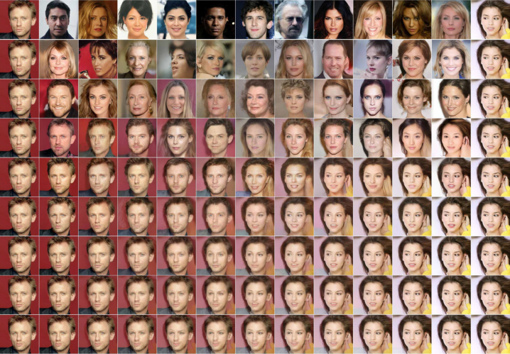
粗到细插值 图 9 显示了当我们改变潜空间插值之前的扩散步数时，一对源 CelebA $256 \times 256$ 图像之间的插值。增加扩散步数会破坏源图像中的更多结构，模型在反向过程中完成这些结构。这允许我们在精细粒度和粗糙粒度上进行插值。在 0 扩散步的极限情况下，插值在像素空间中混合源图像。另一方面，在 1000 扩散步后，源信息丢失，插值成为新样本。